This is a paper experiment. Sample counts, rates, and per-share prices are real numbers from collected data. Account size is not disclosed.
I was hunting for an edge in five-minute up/down rounds on a prediction market. The axis where an LLM called the direction was already dead — 186 actual wins against the 190.8 implied by the market's own ask, z = −0.49. The information the model added on top of the price was zero.
If prediction is dead, the only candidate left is a bias in the price itself. So I backfilled four days — 6,639 rounds across 8 assets — and started scanning a grid. Time-to-expiry buckets × price bands.
In one day I said "found it" three times, and killed it three times myself.
Does your backtest count how many cells it opened before it produced a result?
Death #1: overlapping windows lied about where the signal was
The first find was "the trailing side is overpriced within 60 seconds of expiry." It looked good: monotone growth toward expiry, same sign on all 8 assets.
The problem was how I cut the window.
# what I had labeled "the 60-seconds-to-expiry point"
WHERE p.ts <= r.end_ts - 60 AND p.ts >= r.end_ts - 60 - 90
That is not within 60 seconds of expiry. It is 60 to 150 seconds before it. Cutting three horizons this way made the windows overlap, so the wider one simply contained the narrower one's observations. The label and the contents disagreed.
I recut them so they do not overlap.
| Time left | n | Gain | Day-block CI |
|---|---|---|---|
| 0–60s | 1,616 | +0.0274 | [−0.0051, +0.0521] |
| 60–120s | 2,661 | +0.0260 | [+0.0109, +0.0419] |
| 120–180s | 3,778 | +0.0083 | [−0.0168, +0.0245] |
| 180–240s | 5,044 | −0.0050 | [−0.0145, +0.0070] |
| 240–300s | 5,616 | −0.0110 | [−0.0176, −0.0051] |
The window I had called "just before expiry" — and had already preregistered — was actually one bucket over. Overlapping windows get the size wrong, but worse, they get the location wrong.
Death #2: one asset was making the signal
The freshly cut 0–60s bucket still looked large at +0.0274. So I split it by asset.
The thinnest-liquidity name of the eight came in at +0.1460. The other seven together came to +0.0015. Effectively zero.
Only the 60–120s bucket survived. Excluding that asset it was +0.0227, day-block cluster CI [+0.0080, +0.0404]. All 8 assets positive, 4 of 5 days positive.
This is the one I preregistered. I did the size math first (per-trade ceiling, daily ceiling), then the power math (verdict in 15 days), and attached controls. Procedurally, nothing to complain about.
Would you have stopped here?
The state of things:
- single-cell p = 0.025
- same sign across all 8 assets
- same sign on 4 of 5 days
- spread and overround measured from live quotes; still positive after deducting them
Two ways forward.
- Preregister it and confirm on 15 days of out-of-sample data (what I actually did)
- Before spending those two weeks, interrogate how I found this cell in the first place
Option 1 is not wrong. Out-of-sample eventually tells the truth. It just costs two weeks.
Death #3: I simulated a perfectly efficient market
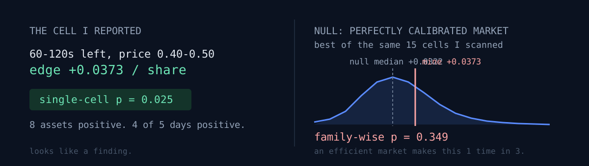
Option 2 turns out to be simple. Set the null to a perfectly efficient market, then scan exactly as many cells as I actually scanned.
# null: the price IS the true probability
outcome = 1 if random.random() < price else 0
# compute all 15 cells I looked at (5 time buckets x 3 price bands)
# and record only the MAXIMUM. Repeat 2,000 times.
The point is that you need the distribution of the maximum, not of one cell. Scanning a grid means the thing I actually do is "pick the best one."
| Value | |
|---|---|
| My best cell (60–120s · 0.40–0.50) | +0.0373 |
| Median of the null maximum | +0.0322 |
| Null 95th percentile | +0.0630 |
| Family-wise p | 0.349 |
| (for reference) single-cell p | 0.025 |
Even in a perfectly efficient market, scanning 15 cells produces something this big one time in three. My value sat in the middle of the null's distribution — barely 0.005 above its median.
And that null ignores cross-asset correlation (all 8 assets move together at the same timestamp, ρ ≈ 0.23), which makes the simulated distribution narrower than reality. So the true p is larger than 0.349.
The single-cell p = 0.025 is not a lie. It is simply a number that is only valid if you named the cell in advance. I did not name it. I found it by scanning.
What I could see once it was dead
Re-reading the same data after rejecting it, three things had been off from the start.
The edge was concentrated in stale quotes. Rounds whose price had not moved at all in the prior minute: +0.1583 (n=56). Barely moved: +0.0518. The properly-moving majority (n=1,067): +0.0227, with a round-cluster CI that includes zero. 27% of the sample was producing 52% of the total edge.
The spread assumptions were, if anything, correct. Collecting live order books separately confirmed a median ask − mid of exactly +0.010 and an overround (both asks summed, minus 1) of +0.020. The arithmetic was right. What was missing was the edge that fed into it.
The mechanism did not explain the shape. If the story is "the market underprices time decay near expiry," the values should increase monotonically. Actual: 120–180s +0.027 → 60–120s +0.037 → 0–60s +0.002. It exists in exactly one bucket. No mechanism predicts that shape. Only noise does.
A three-line self-check
Run these against your current backtest.
- Did you count how many cells you opened? Multiply your parameter, window, and filter choices — that product is how many tests you actually ran. Simulate the null that many times and plot the distribution of the maximum. It is about twenty lines of code.
- Do your windows overlap? Overlapping windows misreport the location of a signal, not just its size. Recut them disjointly and check whether the number survives.
- Does it collapse if you drop one? Rerun without one asset, and without one day. I have had a signal that a single name was generating on its own.
The honest part
This axis is closed. Prediction (LLM), price bias, model (diffusion fair value), and exit policy — four branches, nothing left. A full day of digging produced "there is nothing here."
But making the same class of mistake three times in one day and catching all three was worth more than the result. What remains is three reusable tools: a family-wise p simulator, a disjoint-bucket splitter, and a two-level (round / day) cluster bootstrap. The next experiment starts holding these.
Preregistration is the habit of writing the rules before you see the data. This time I learned its counterpart. If you found something after looking at the data, you also have to write down how many times you looked. Without that number, the p-value means nothing. The one where the measurement itself only counted winners and the one about killing failed bots cleanly are the same story wearing different faces.
How many combinations did your last backtest actually run? I would like to know the number.